The Yin and Yang of Finance: A Closer Look at the Stock-Bond Relationship

As both stocks and bonds are two major asset classes playing an important role in asset allocation, their relationship has garnered considerable interest among portfolio managers. The tendency on how the return of one asset moves in tandem with the other, also called correlation, provides strategic information for dynamic asset allocation, resulting in better hedging choices, risk management and portfolio optimization.

 

1. Embracing the Dynamic Stock-Bond Return Correlation

Stock and bond prices are driven by common factors such as interest rates, economic conditions, investor sentiment, financial market uncertainty, … These common factors and their impact on stock and bond prices vary over time, implying that the stock-bond return correlation should have a time-varying character. This article examines the historical dynamics of the stock-bond return correlation using empirical evidence and a dynamic correlation model. It also demonstrates how investors can capitalize on asset class diversification during periods of financial market uncertainty.

 

 

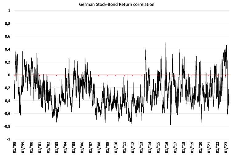
Source: This figure shows the dynamic stock-bond return correlation between the Dax Total Return Index and the Thomson Reuters Generic 10-Year German Government Benchmark in the period 01/01/1998-05/06/2023. Correlations are estimated using an ADCC-GARCH(1,1) model. The DAX index serves as a proxy for stock returns, the Thomson Reuters benchmark serves as a proxy for bond returns. Data frequency is daily. With the exception of this figure, the price evolution of the Dax Index and Thomson Reuters Generic 10-Year German Government Benchmark, all figures below are plotted as 40-day Moving Averages which allows for better graphing and interpretation.

The figure presented above illustrates the dynamic changes in the relationship between stock and bond returns since January 1998. The correlation, displayed on a scale of -1 to 1, represent the strength of the relationship between the two. A correlation of -1 means that stock and bond returns perfectly move in opposite directions, while a correlation of 1 means that stock and bond returns perfectly move in the same direction. When the correlation is close to 0, no clear relationship between stock and bond returns exists. The data clearly shows that the stock-bond relationship has not been constant over time, but instead exhibits a varying nature. This finding suggests that actively managing a portfolio and making dynamic adjustments to  asset class allocations can be highly beneficial.

Historically, stock and bond returns have displayed a negative correlation. Throughout the observation period,the average stock-bond return correlation has been -0.26.  This negative correlation offers a potential balancing effect within an investor’s portfolio. Positive returns in one asset class are partially offset by negative returns in the other, and vice-versa. While this suggests a diversification benefit, it does not necessarily indicate the presence of diversification during times when it is truly needed, namely in times of financial market uncertainty.

 

 

1.1. Russian Ruble Crash

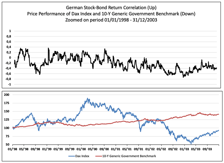
In August 1998, Russia experienced a severe financial crisis that had far-reaching consequences. The crisis involved the devaluation of the Russian ruble, a default on its sovereign debt, and a 90-day suspension on payments by commercial banks to foreign creditors. This crisis had a significant impact on global financial markets. Russia’s sovereign default at that time was the largest in history at the time and had repercussions, including the collapse of the LTCM hedge fund in the United States. This led to substantial spillover effects in international markets. During this crisis, fear among investors grew, prompting a flight from risky assets such as equities to safer government bonds. This flight-to-quality event resulted into correlations plummeting into negative territory.

1.2. Dotcom Bubble Burst

Another flight-to-quality event took place during the Dotcom bubble burst, although it occurred over a longer time span compared to the Russian Ruble Crash. The American Federal Reserve increased interest rates multiple times in the early 2000s. This series of rate increases, in combination with news of Japan entering a recession, triggered a global sell-off in both bonds and equities. Nn such a dash-for cash event, stock-bond return correlations tend to be positive.

Subsequently, as the Dotcom bubble burst, investors began to reassess the risks associated with stocks, particularly those in the technology sector. The sharp decline in stock prices eroded investor confidence and increased their risk aversion, resulting in investors seeking safer investments such as government bonds. Central banks responded to the bursting of the dotcom bubble by cutting interest rates aimed at stimulating investment and consumption. These actions had an impact on both stock and bond markets. While the interest rate cuts aimed to stimulate stock markets, the flight to safety towards bonds persisted. As a result, bond prices increased following the central banks’ rate cuts. This process of risk reevaluation, rate cuts and the subsequent flight from stocks to bonds led to negative correlations during this period of financial market stress.

1.3. Global Financial Crisis

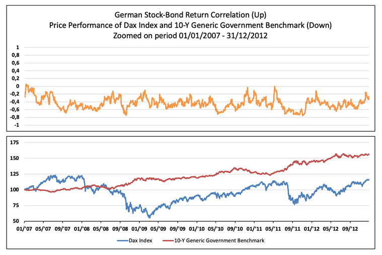
During the global financial crisis, the correlation between stock and bond returns underwent notable changes. The crisis, triggered by the collapse of the US housing market and the subsequent ripple effects on the global banking system, created an environment of increased risk aversion and widespread economic uncertainty. This uncertainty, together with concerns about the solvency of financial institutions, led to significant declines in stock prices. On the other hand, government bonds, particularly those issued by countries with stronger credit ratings, were seen as relatively safe, stable and less exposed to the risks associated with the crisis. Central banks worldwide implemented unconventional monetary policy measures to address the financial crisis. These measures included interest rate cuts, large-scale asset purchases (quantitative easing), and liquidity provision to stabilize the financial system. Bond prices were positively impacted as central banks purchased bonds, while stock prices struggled amid ongoing economic challenges. The figure given above illustrates the overall negative correlations during the stock market fall over January 2008 – October 2008. In hindsight, an investor might have effectively hedged his equity exposure with government bonds due to the negative return correlations.

1.4. Covid-19

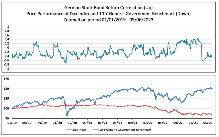
At the beginning of March 2020, correlations between stocks and bond returns plunged into deep negative territory. This occurred as investors swiftly exited the equity market exits and sought refuge in safe haven assets. Consequently, 10-year government bond prices rose while stock prices tumbled. In the second week of March 2020, a short dash-for-cash event took place. During this period, investors sold both bonds and equities to meet redemptions and margin calls, reduce leverage, and build up cash buffers. The stock-bond return correlation quickly reversed from -0.5 levels to positive territory.

1.5. Russian Invasion of Ukraine

The frequent occurrence of negative correlations during periods of financial market stress could suggest that stock market losses are usually offset by bond market gains, and vice-versa. Together with some historic short-term dash-for-cash events, the prolonged Russian-Ukrainian war has shown a long period of negative contagion. In a negative contagion event, the prices of both stocks and bonds decrease, leading to positive correlations between their returns. Government bonds initially were a hiding place in the stock market sell-off in February-March 2022, with correlations being around the -0,5 level. Thereafter, a mix of economic and geopolitical uncertainty, followed by central banks’ rate hikes in order to battle inflation, influenced prices in both the stock and bond markets. A long period of positive correlations was the result of both positive as negative contagion events following up on each other. In periods of contagion, mixed funds that combine both stocks and bonds do not provide the benefit of diversification originating from negatively correlated assets. This highlights the importance of understanding the changing dynamics of correlations between stocks and bonds during times of financial stress.

 

2. Unveiling Lessons from the Historical Relationship

It is evident that during various financial market stress events, investor have sought a place to hide. Government bonds of countries with favorable credit ratings are typically perceived as low risk assets. This perception, in combination with central banks often lowering their target rates in times of financial market turmoil, made bonds deliver positive returns while stock markets saw losses. However, government bonds do not dilute equity risk in times of negative contagion. In short, following cheat sheet can be used to see how the correlations relate to what is happening in the markets:  

	Stock Market Up	Stock Market Down
Positive Correlation	Positive Contagion  (Bond Market Up)	Negative Contagion (Bond Market Down)
Negative Correlation	Flight-from-quality (Bond Market Down)	Flight-to-quality (Bond Market Up)

Assuming that stock-bond return correlations are dynamic rather than static, allows for dynamic and active decision making. This approach enables portfolio manager to adjust their exposure to safer assets when markets start to rumble and increase their exposure to riskier assets in times of financial market flourishment. History has proven this to be a succesfull strategy, but just as past returns are no guarantee of future performance, the same applies to past correlations. The Russian-Ukrainian war serves as a prime example in this context. The question that remains is whether stock-bond return correlations can be utilized to help make decisions about asset class distributions.

 

 

3. A word on dynamic hedge ratios and weight distributions

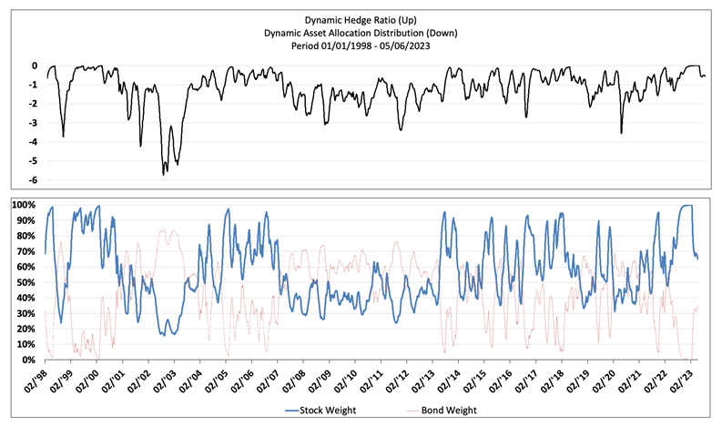
When considering correlations as measures both stocks and government bonds volatilities, it is possible to construct a dynamic optimal hedge ratio. This optimal hedge ratio can then be utilized  to determine a dynamic weight allocation between stock and bonds within a mixed portfolio aiming for minimum variance. A quantitative model, based on several assumptions, could be a great addition to qualitative decision making. Referring to the given figure above, a hedge ratio of -2 can be interpreted as: “In a minimum volatility portfolio, an equity exposure of €1 is hedged by a bond exposure of €2.” Therefore, a more negative hedge ratio indicates a greater allocation to government bonds in order to achieve the minimum-variance portfolio. Notably, the model demonstrates the ability to capture financial market stress events by reflecting a flight-to-quality and reporting lower hedge ratios during such periods. Conversely, during stock market growth phases, the model tends to increase the equity weight. However, the extent to which this dynamic weight allocation decision can effectively reduce portfolio volatility remains a questions that requires further examination.

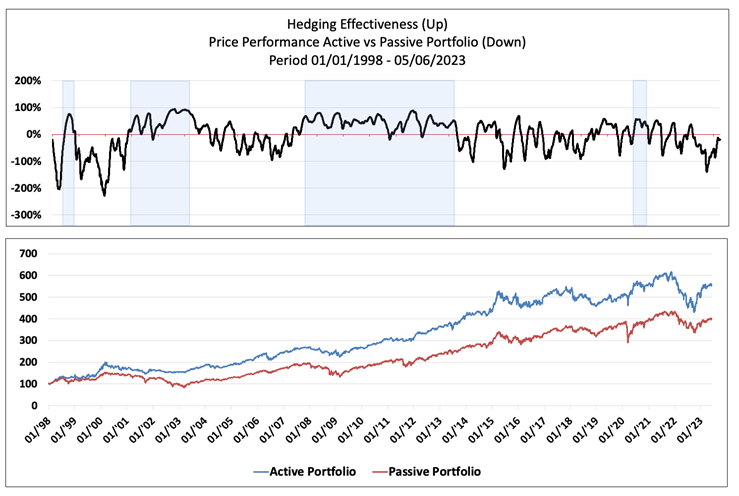
4. Hedging Effectiveness

In the above figure, the actively managed portfolio, based on a correlation model-derived hedge ratios, is compared to a passive fixed weight portfolio. The passive fixed weight portfolio maintains a fixed weight of 60% in stocks and 40% in bonds. The hedging effectiveness represents the percentage of variance reduction when comparing the active portfolio to the fixed portfolio. A positive value, such as 50%, indicates that the active portfolio has a 50% lower variance (and thus lower volatility) than the fixed weight portfolio. Conversely, a negative percentage means that the active portfolio was more volatile than the fixed portfolio.

 

It is important to note that hedging effectiveness is desired in times that it is needed the most: periods of financial market turmoil. The hedging effectiveness graph clearly shows effective hedging (positive numbers) in the Russian Ruble crash, the dotcom bubble, the Global Financial Crisis and the Covid-19 crisis. However, the model reveals its limitations during the contagion event triggered by the Russian invasion of Ukraine, both in terms of performance and volatility reduction. Over the entire observation window, active portfolio management has proved to be effective both in terms of volatility and performance*.

 

When combined with qualitative decision-making concerning future financial market evolutions, a quantitative dynamic correlation model, that constructs a risk-minimizing weight distribution, can be of great value.

* Performance does not take into account transaction costs of hedging.
Click here for more information on the methodology used in this article.